6  美国大规模枪击案

6.1 变量说明

变量说明。

6.2 描述性分析

shoot <- read_csv("data/Mass shooting/Mass Shootings Dataset Ver 3.csv")
shoot <- shoot %>% 
  rename(ID = `S#`, Open_Close = `Open/Close Location`,
         Total = `Total victims`,
         Mental = `Mental Health Issues`)
shoot$Date <- as.Date(shoot$Date, "%m/%d/%Y")
shoot$year <- year(shoot$Date)
shoot <- shoot %>% 
  filter(year != 1966)

glimpse(shoot)

Rows: 318
Columns: 22
$ ID                 <dbl> 1, 2, 3, 4, 5, 6, 7, 8, 9, 10, 11, 12, 13, 14, 15, …
$ Title              <chr> "Las Vegas Strip mass shooting", "San Francisco UPS…
$ Location           <chr> "Las Vegas, NV", "San Francisco, CA", "Tunkhannock,…
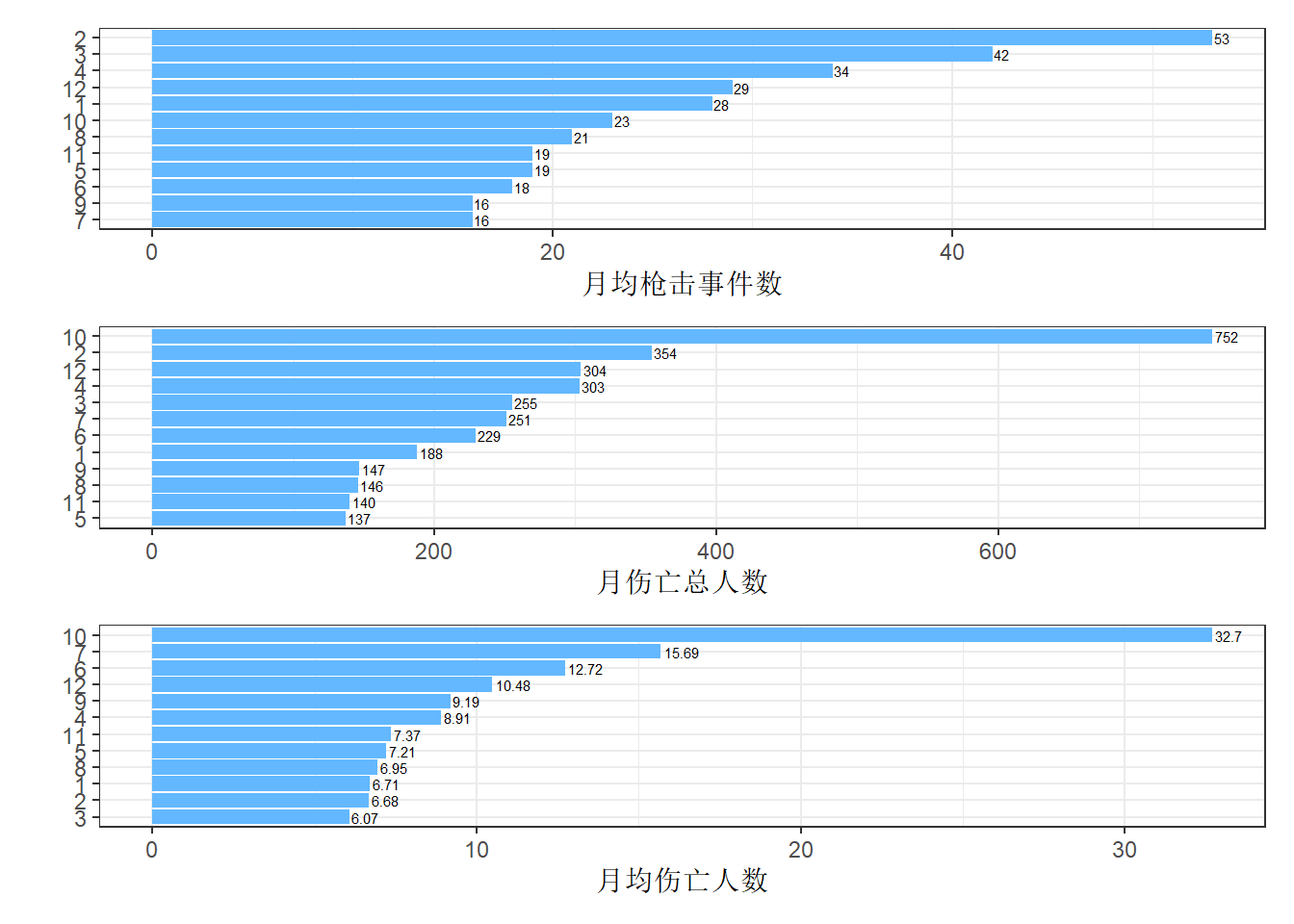
$ Date               <date> 2017-10-01, 2017-06-14, 2017-06-07, 2017-06-05, 20…
$ `Incident Area`    <chr> NA, "UPS facility", "Weis grocery", "manufacturer F…
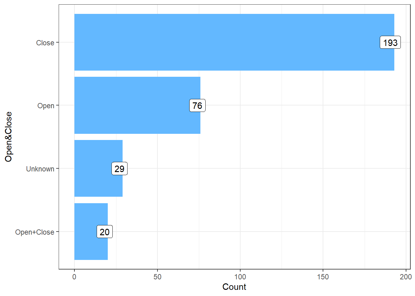
$ Open_Close         <chr> NA, "Close", "Close", "Close", "Close", "Open", "Cl…
$ Target             <chr> NA, "coworkers", "coworkers", "coworkers", "coworke…
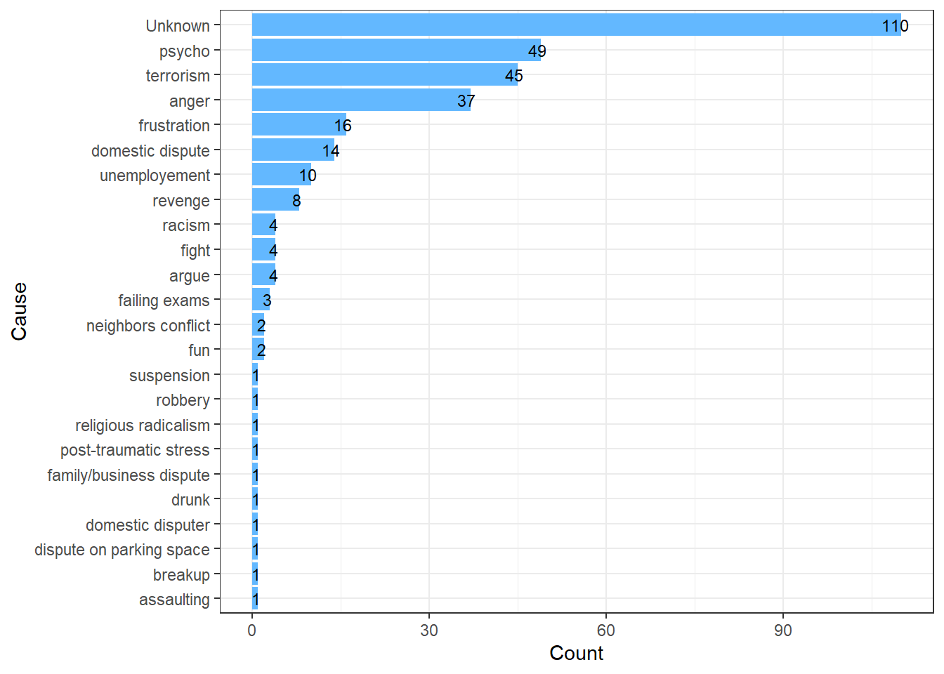
$ Cause              <chr> NA, NA, "terrorism", "unemployement", NA, "racism",…
$ Summary            <chr> NA, "Jimmy Lam, 38, fatally shot three coworkers an…
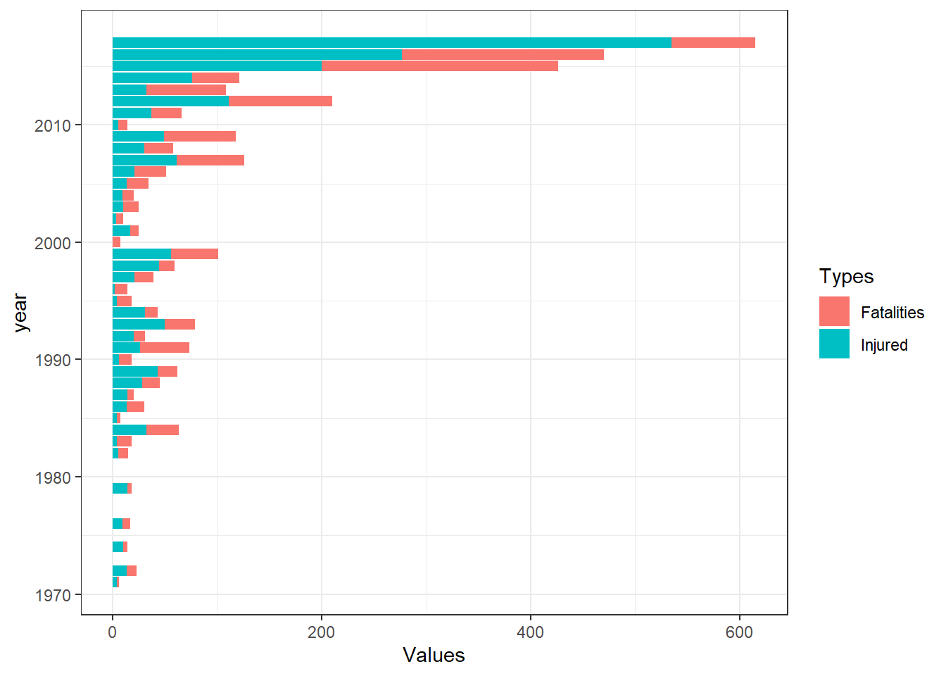
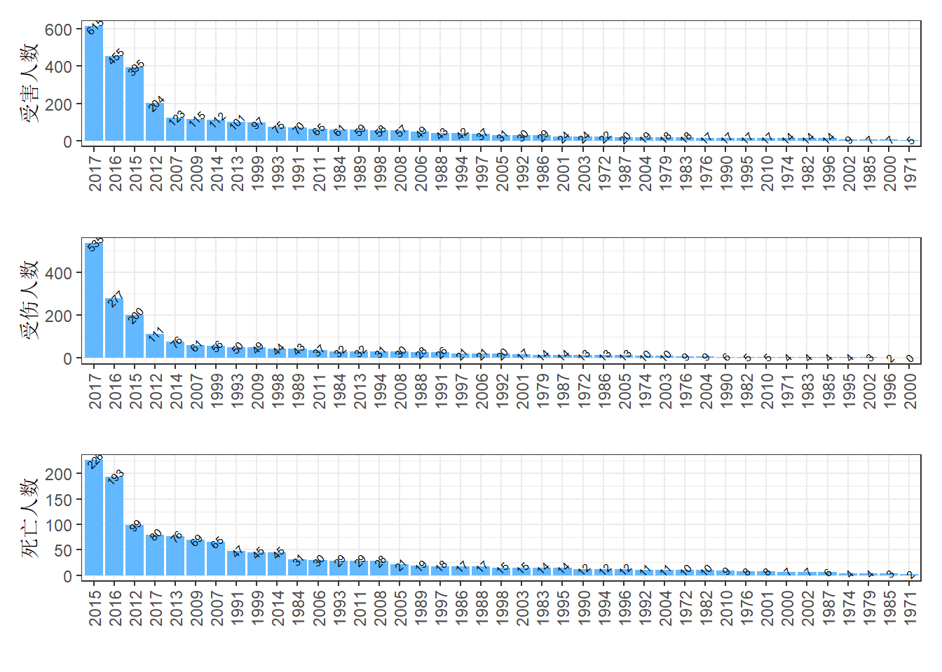
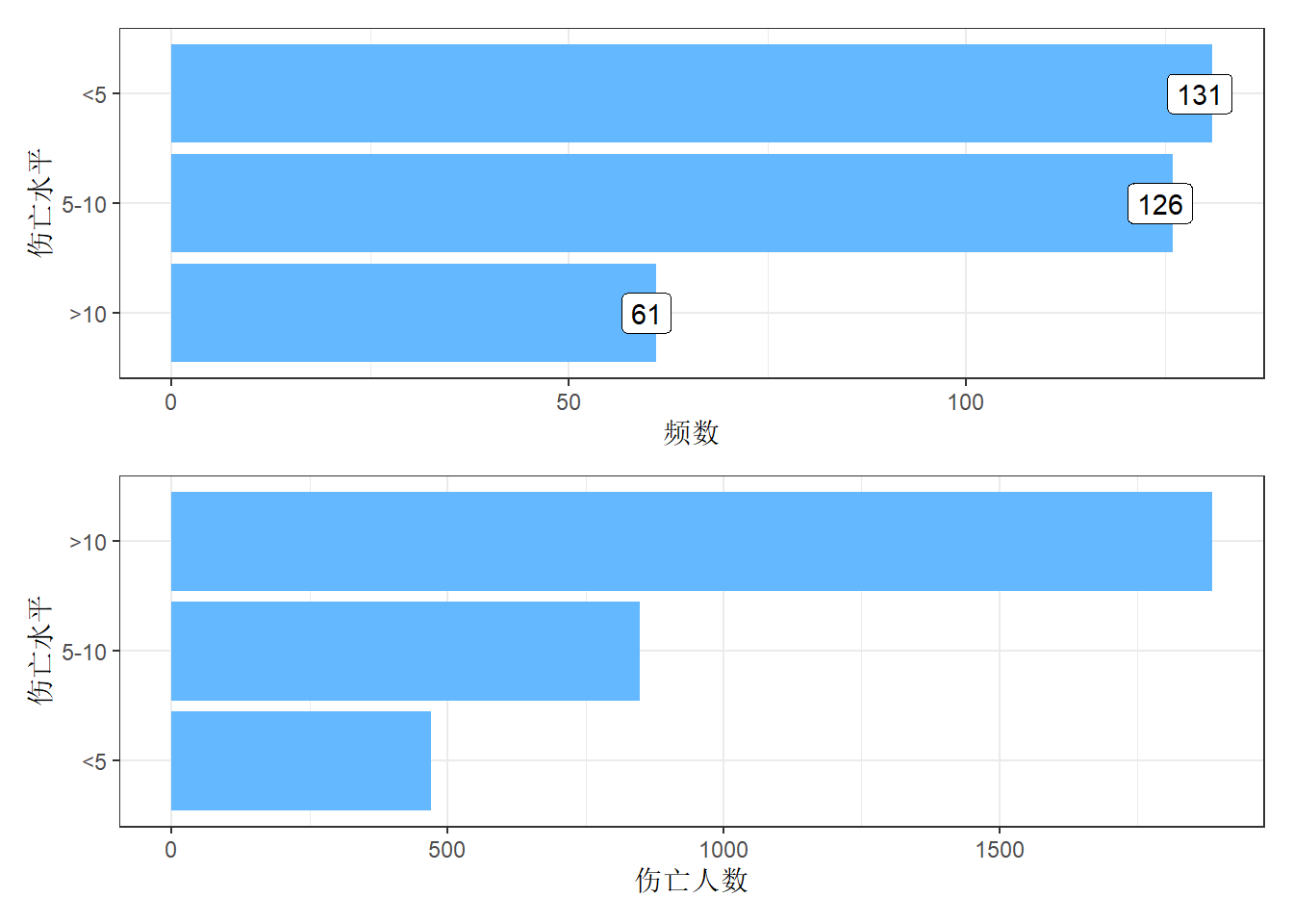
$ Fatalities         <dbl> 58, 3, 3, 5, 3, 3, 5, 5, 3, 5, 49, 0, 1, 0, 0, 1, 4…
$ Injured            <dbl> 527, 2, 0, 0, 0, 0, 6, 0, 3, 11, 53, 4, 4, 6, 4, 4,…
$ Total              <dbl> 585, 5, 3, 5, 3, 3, 11, 5, 6, 16, 102, 4, 5, 6, 4, …
$ `Policeman Killed` <dbl> NA, 0, NA, NA, 1, NA, NA, NA, 3, 5, 0, 0, 0, 0, 0, …
$ Age                <dbl> NA, 38, 24, 45, 43, 39, 26, 20, NA, 25, 29, 0, NA, …
$ `Employeed (Y/N)`  <dbl> NA, 1, 1, 1, 1, NA, NA, NA, NA, NA, NA, NA, NA, NA,…
$ `Employed at`      <chr> NA, NA, "Weis grocery", "manufacturer Fiamma Inc.",…
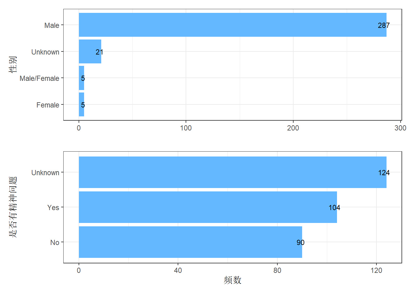
$ Mental             <chr> "Unclear", "Yes", "Unclear", "Unclear", "Yes", "Unc…
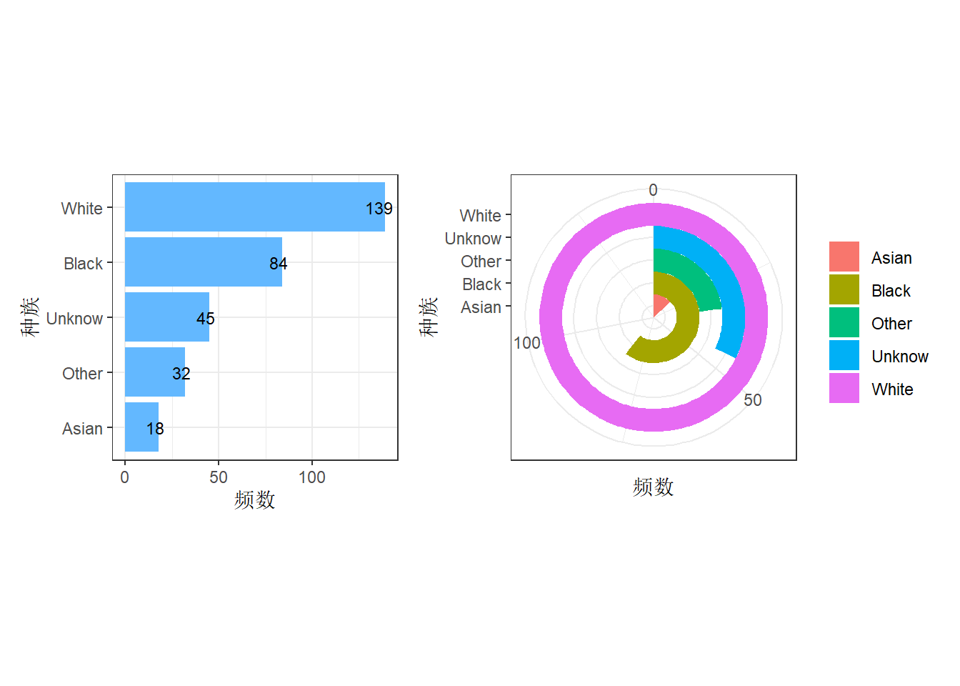
$ Race               <chr> "White", "Asian", "White", NA, "White", "Black", "L…
$ Gender             <chr> "M", "M", "M", "M", "M", "M", "M", "M", "M", "M", "…
$ Latitude           <dbl> 36.18127, NA, NA, NA, NA, NA, NA, NA, NA, NA, NA, 3…
$ Longitude          <dbl> -115.13413, NA, NA, NA, NA, NA, NA, NA, NA, NA, NA,…
$ year               <dbl> 2017, 2017, 2017, 2017, 2017, 2017, 2017, 2016, 201…

6.2.1 枪击案中伤亡人数

# 封装条形图作图函数
fun_bar1 <- function(data, xlab, ylab, xname, yname){
  data %>% 
    group_by({{xlab}}) %>% 
    summarise(count = sum({{ylab}})) %>% 
    ggplot(aes(x = reorder(year, -count),
               y = count)) +
      geom_bar(stat = "identity", fill = "#63B8FF") +
      labs(x = xname, y = yname) +
      theme_bw() +
      theme(axis.text.x = element_text(angle = 90, vjust = 0.5))
}

p1 <- fun_bar1(shoot, year, Total, " ", "受害人数") +
  geom_text(aes(label = count), size = 2, angle = 45, vjust = 0.5)

p2 <- fun_bar1(shoot, year, Injured, " ", "受伤人数")+
  geom_text(aes(label = count), size = 2, angle = 45, vjust = 0.5)

p3 <- fun_bar1(shoot, year, Fatalities, " ", "死亡人数")+
  geom_text(aes(label = count), size = 2, angle = 45, vjust = 0.5)

shoot %>% 
  select(year, Injured, Fatalities) %>% 
  pivot_longer(-year,
               names_to = "Types",
               values_to = "Values") %>% 
  ggplot(aes(x = year,  y = Values, fill = Types)) +
    geom_col() +
    coord_flip() +
    theme_bw() 

p1/p2/p3

• 整体而言，总伤亡人数呈现增长趋势。

• 2015-2017年间，伤亡人数突然增多。

• 受害人数2017年最多，1971年最少。

• 除2017年外，其余年份受伤和死亡任务相对平衡

6.2.2 绘制枪击案频率、伤亡总人数和平均伤亡人数（月为单位）

# 提取月份数据
shoot$month <- month(shoot$Date)

# 每月枪击频率
p4 <- month_freq <- shoot %>% 
  group_by(month) %>% 
  summarise(freq = n()) %>% 
  ggplot(aes(x = reorder(month, freq), y = freq)) +
    geom_bar(stat = "identity", fill = "#63B8FF") +
    geom_text(aes(label = freq), hjust = -0.1, size = 2) +
    labs(x = " ", y = "月均枪击事件数") +
    coord_flip() +
    theme_bw()

# 月伤亡总人数
p5 <- month_total <- shoot %>% 
  group_by(month) %>% 
  summarise(total = sum(Total))%>% 
  ggplot(aes(x = reorder(month, total), y = total)) +
    geom_bar(stat = "identity", fill = "#63B8FF") +
    geom_text(aes(label = total), hjust = -0.1, size = 2) +
    labs(x = " ", y = "月伤亡总人数") +
    coord_flip() +
    theme_bw()

# 月均伤亡人数
p6 <- month_meantotal <- shoot %>% 
  group_by(month) %>% 
  summarise(mean = mean(Total)) %>% 
  ggplot(aes(x = reorder(month, mean), y = mean)) +
    geom_bar(stat = "identity", fill = "#63B8FF") +
    geom_text(aes(label = round(mean,2)), hjust = -0.1, size = 2) +
    labs(x = " ", y = "月均伤亡人数") +
    coord_flip() +
    theme_bw()
p4/p5/p6 

绘制枪击案频率、伤亡总人数和平均伤亡人数（月为单位）

• 十月份至少发生过一起大型枪击案

6.2.3 枪手与种族之间的关系

table(shoot$Race)

                                              Asian 
                                                  6 
                                     Asian American 
                                                 11 
                     Asian American/Some other race 
                                                  1 
                                              black 
                                                  3 
                                              Black 
                                                  4 
                 Black American or African American 
                                                 76 
         Black American or African American/Unknown 
                                                  1 
                                             Latino 
                                                  5 
                   Native American or Alaska Native 
                                                  3 
                                              Other 
                                                  2 
                                    Some other race 
                                                 20 
                                  Two or more races 
                                                  2 
                                            Unknown 
                                                 42 
                                              white 
                                                 12 
                                              White 
                                                  7 
                White American or European American 
                                                120 
White American or European American/Some other Race 
                                                  1 

# 将所有重复的数据重塑为统一
shoot <- within(shoot,{ 
  Race_new <- " "
  Race_new[Race == "Black"|
             Race == "black"|
             Race == "Black American or African American"|
             Race == "Black American or African American/Unknown"] <- "Black"
  Race_new[Race == "White"|Race == "white"|
             Race == "White American or European American"|
             Race == "White American or European American/Some other Race "] <- "White"
  Race_new[Race == "unclear"|
             Race == ""|
             Race == "Unknown"] <- "Unknow"
  Race_new[Race == "Asian"|
             Race == "Asian American/Some other race"|
             Race == "Asian American"] <- "Asian"
  Race_new[Race == "Latino"|Race == "Other"|
             Race == "Native American or Alaska Native"|
             Race == "Native American"|
             Race == "Some other race"|
             Race == "Two or more races"] <- "Other"
})

# 统计不同Race_new的个数
shoot$Race_new[is.na(shoot$Race_new)] <-  "Unknow"
p7 <- shoot %>% 
  group_by(Race_new) %>% 
  summarise(freq = n()) %>% 
  ggplot(aes(x = reorder(Race_new, freq), y = freq)) +
    geom_bar(stat = "identity", fill = "#63B8FF") +
    geom_text(aes(label = round(freq, 2)), hjust = 0.7, size = 3) +
    labs(x = "种族", y = "频数") +
    coord_flip() +
    theme_bw()
p8 <- shoot %>% 
  group_by(Race_new) %>% 
  summarise(freq = n()) %>% 
  ggplot(aes(x = Race_new, y = freq, fill = Race_new)) +
    geom_bar(stat = "identity", width = 1) +
    labs(x = "种族", y = "频数") +
    coord_polar(theta = "y") + # 将角度映射到y轴
    theme_bw() +
    guides(fill = guide_legend(title = NULL))
p7|p8

枪手与种族之间的关系

• 枪手中白种人最多，黑种人次之，亚洲人最少。

6.2.4 杀手性别和精神状况

# 性别情况
table(shoot$Gender)

     Female           M         M/F        Male Male/Female     Unknown 
          5          17           1         270           4          21 

# 对数据进行重塑统一
shoot$Gender[shoot$Gender == "M"] <- "Male"
shoot$Gender[shoot$Gender == "M/F"] <- "Male/Female"

p9 <- shoot %>% 
  group_by(Gender) %>% 
  summarise(count = n()) %>% 
  ggplot(aes(x = reorder(Gender, count), y = count)) +
    geom_bar(stat = "identity", fill = "#63B8FF") +
    geom_text(aes(label = count), hjust = 0.7, size = 3) +
    labs(x = "性别", y = " ") +
    coord_flip() +
    theme_bw()

# 精神情况
table(shoot$Mental)

     No Unclear unknown Unknown     Yes 
     90      13       1     110     104 

shoot$Mental[shoot$Mental == "Unclear"|
               shoot$Mental == "Unknown"|
               shoot$Mental == "unknown"] <- "Unknown"

p10 <- shoot %>% 
  group_by(Mental) %>% 
  summarise(count = n()) %>% 
  ggplot(aes(x = reorder(Mental, count), y = count)) +
    geom_bar(stat = "identity", fill = "#63B8FF") +
    geom_text(aes(label = count), hjust = 0.7, size = 3) +
    labs(x = "是否有精神问题", y = "频数") +
    coord_flip() +
    theme_bw()

p9/p10

杀手性别和精神状况

由图@ref(fig:gender-mental)可知：

• 枪手中男性占绝大多数。

• 并不是每个枪手都有精神问题，相反有精神问题的与没有精神问题的枪手数量并未拉开差距。

6.2.5 伤亡水平和不同伤亡水平伤亡人数

# 按照伤亡人数确定伤亡水平
shoot <- within(shoot,{
  level <- ""
  level[Total < 5] <- "<5"
  level[Total>=5] <- "5-10"
  level[Total>10] <- ">10"
})

p11 <- shoot %>% 
  group_by(level) %>% 
  summarise(count = sum(Total)) %>% 
   ggplot(aes(x = reorder(level, count), y = count)) +
    geom_bar(stat = "identity", fill = "#63B8FF") +
    #geom_label(aes(label = level), hjust = 0.7) +
    labs(x = "伤亡水平", y = "伤亡人数") +
    coord_flip() +
    theme_bw()

p12 <- shoot %>% 
  group_by(level) %>% 
  summarise(count = n()) %>% 
   ggplot(aes(x = reorder(level, count), y = count)) +
    geom_bar(stat = "identity", fill = "#63B8FF") +
    geom_label(aes(label = count), hjust = 0.7) +
    labs(x = "伤亡水平", y = "频数") +
    coord_flip() +
    theme_bw()
p12/p11

伤亡水平和不同伤亡水平伤亡人数

由图@ref(fig:casualties-level)可知：

• 大部分枪击事件为伤亡人数5-10之间的小规模枪击事件。

• 伤亡水平大于10的案件中总伤亡人数远多于小伤亡水平的枪击案件。

6.3 枪击发生地的可视化（地图）

states_map <- map_data("state") # 获取美国地图
p13 <- ggplot() +
  geom_polygon(data= states_map, 
               aes(x = long, y = lat, group = group),
               color = "black", fill = "white") +
  geom_point(data = shoot[shoot$Longitude >= -140, ],
             aes(x = Longitude, y = Latitude,
             size = Total, color = Fatalities), 
             alpha = 0.6) +
  scale_color_gradient(low = "red", high = "black")
ggplotly(p13)

• 枪击案多发生在美国东部地区及西部边境地区。

6.4 枪击案发生地点（是否露天）

table(shoot$Open_Close)

     Close       Open Open+Close Open+CLose 
       193         76         19          1 

shoot$Open_Close[is.na(shoot$Open_Close)] <- "Unknown"
shoot$Open_Close[shoot$Open_Close == "Open+CLose"] <- "Open+Close"

shoot_Op_Cl <- shoot %>% 
  group_by(Open_Close) %>% 
  summarise(Count = n())

P14 <- ggplot(shoot_Op_Cl, aes(x = reorder(Open_Close, Count), y = Count))+
  geom_col(fill = "#63B8FF") +
  geom_label(aes(label = Count), hjust = 0.7) +
  coord_flip()+
  labs(x = "Open&Close", y = "Count") +
  theme_bw()
P14

• 枪击案件大多发生在室内，室外枪击的数量不到室内数量的一半。

6.5 不同枪击案起因

shoot_cause <- shoot %>% 
  group_by(Cause) %>% 
  summarise(Count = n())

shoot_cause$Cause[is.na(shoot_cause$Cause)] <- "Unknown"

(P15 <- ggplot(shoot_cause, aes(x = reorder(Cause, Count), y = Count))+
  geom_col(fill = "#63B8FF") +
  geom_text(aes(label = Count), hjust = 0.7, size = 3) +
  coord_flip()+
  labs(x = "Cause", y = "Count") +
  theme_bw())

• 枪击案的发生大都由于枪手存在精神问题。

• 恐怖主义、愤怒和挫折是除精神问题外引发枪击案最多的诱因。