1 Video Games Sales

1.1 准备

file <- "D:/Tools/Rwork/0.Study R/kaggle-project/data/vgsales.csv"
df <- read_csv(file)
str(df)

spec_tbl_df [19,600 × 9] (S3: spec_tbl_df/tbl_df/tbl/data.frame)
 $ Rank         : num [1:19600] 1 2 3 4 5 6 7 8 9 10 ...
 $ Name         : chr [1:19600] "Wii Sports" "Super Mario Bros." "Counter-Strike: Global Offensive" "Mario Kart Wii" ...
 $ Platform     : chr [1:19600] "Wii" "NES" "PC" "Wii" ...
 $ Publisher    : chr [1:19600] "Nintendo" "Nintendo" "Valve" "Nintendo" ...
 $ Developer    : chr [1:19600] "Nintendo EAD" "Nintendo EAD" "Valve Corporation" "Nintendo EAD" ...
 $ Critic_Score : num [1:19600] 7.7 10 8 8.2 8.6 10 8 9.4 9.1 8.6 ...
 $ User_Score   : num [1:19600] 8 8.2 7.5 9.1 4.7 7.8 8.8 8.8 8.1 9.2 ...
 $ Total_Shipped: num [1:19600] 82.9 40.2 40 37.3 36.6 ...
 $ Year         : num [1:19600] 2006 1985 2012 2008 2017 ...
 - attr(*, "spec")=
  .. cols(
  ..   Rank = col_double(),
  ..   Name = col_character(),
  ..   Platform = col_character(),
  ..   Publisher = col_character(),
  ..   Developer = col_character(),
  ..   Critic_Score = col_double(),
  ..   User_Score = col_double(),
  ..   Total_Shipped = col_double(),
  ..   Year = col_double()
  .. )
 - attr(*, "problems")=<externalptr>

head(df, 3)

# A tibble: 3 × 9
   Rank Name  Platform Publisher Developer Critic_Score User_Score Total_Shipped
  <dbl> <chr> <chr>    <chr>     <chr>            <dbl>      <dbl>         <dbl>
1     1 Wii … Wii      Nintendo  Nintendo…          7.7        8            82.9
2     2 Supe… NES      Nintendo  Nintendo…         10          8.2          40.2
3     3 Coun… PC       Valve     Valve Co…          8          7.5          40  
# … with 1 more variable: Year <dbl>

数据共包括11列，包含了从1977年~2020年中的游戏销量数据，具体变量说明如下表所示：

table_var <- read_excel("data-intro.xlsx", sheet = 3)
kable(table_var, align = "c") %>% 
  kable_classic()

变量	说明
Rank	销量排名
Name	游戏名称
Platform	发型平台
Publisher	发行商
Develooper	开发商
Critic_Score	从业人评分
User_Score	用户评分
Total_shipped	总销量(百万套)
Year	发型年份

1.2 缺失值处理

summary(df)

      Rank           Name             Platform          Publisher        
 Min.   :    1   Length:19600       Length:19600       Length:19600      
 1st Qu.: 4899   Class :character   Class :character   Class :character  
 Median : 9798   Mode  :character   Mode  :character   Mode  :character  
 Mean   : 9799                                                           
 3rd Qu.:14698                                                           
 Max.   :19598                                                           
                                                                         
  Developer          Critic_Score      User_Score     Total_Shipped    
 Length:19600       Min.   : 0.800   Min.   : 1.000   Min.   : 0.0100  
 Class :character   1st Qu.: 6.100   1st Qu.: 6.300   1st Qu.: 0.0500  
 Mode  :character   Median : 7.300   Median : 7.200   Median : 0.1600  
                    Mean   : 7.035   Mean   : 6.995   Mean   : 0.5511  
                    3rd Qu.: 8.200   3rd Qu.: 8.000   3rd Qu.: 0.4600  
                    Max.   :10.000   Max.   :10.000   Max.   :82.9000  
                    NA's   :9631     NA's   :17377                     
      Year     
 Min.   :1977  
 1st Qu.:2004  
 Median :2008  
 Mean   :2008  
 3rd Qu.:2012  
 Max.   :2020

sum(is.na(df))

[1] 27010

n_miss(df)

[1] 27010

数据中有27010个缺失值，而缺失值主要存在与Critic_Score和User_Score，主要原因在于并不是每个用户和从业者都会对游戏进行评分。需要对其进行一些处理，未打分的我们认为其打分为5.0分，即使用5.0代替所有缺失值。

# 采用每一列的众数替换该列的缺失值
df <- df %>% 
  map_dfc(~replace_na(.x, rstatix::get_mode(.x)[1]))

1.3 描述性分析

描述性统计是一个统计范围，它应用各种技术来描述和总结任何数据集，并研究观察到的数据的一般行为，以促进问题的解决。这可以通过频率表、图形和集中趋势的度量来完成，例如平均值、中位数、众数、离散度量（例如标准偏差、百分位数和四分位数）。

由于2020年只有前半段的数据，我们分析时将2020年的数据剔除，以便更好的分析对比各年份的差异。同时剔除Rank列。

df <- df %>% 
  filter(Year != 2020) %>% 
  select(-Rank)

df$Year <- factor(df$Year)

1.3.1 常规分析

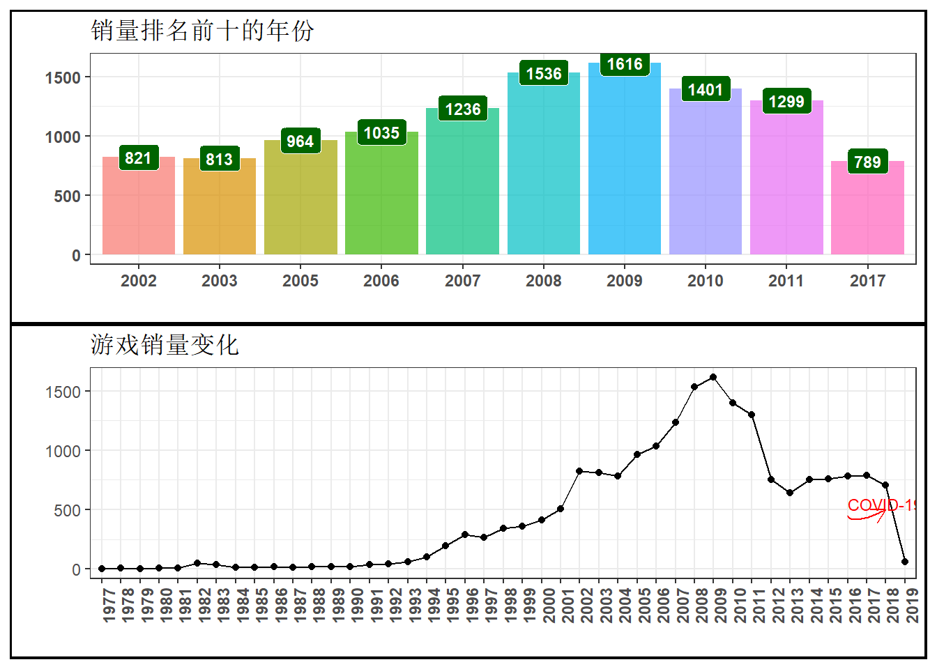
1.3.1.1 哪一年的游戏总销量最高

df_shipped <- df %>% 
  select(Year, Total_Shipped) %>% 
  group_by(Year) %>% 
  summarise(count = n()) %>% 
  arrange(desc(count))

p1 <- ggplot(head(df_shipped,10), aes(x = Year, y = count, 
                       fill = Year)) + 
  geom_bar(stat = "identity", alpha = 0.7) +
  geom_label(aes(label = count), fontface = "bold",
             fill = "#006400", 
             color = "white",
             size = 3) +
  theme_bw() +
  labs(x = " ", y = " ") +
  ggtitle("销量排名前十的年份") +
  theme(legend.position = "none", 
        plot.background = element_rect(color = "black", size = 1.1), 
        axis.text.x = element_text(face = "bold"),
        axis.text.y = element_text(face = "bold"),
        axis.title = element_text(face = "bold")
        )

p2 <- ggplot(df_shipped, aes(x = Year, y = count, group = 1)) +
  geom_point() +
  geom_line() +
  theme_bw() +
  ggtitle("游戏销量变化") +
  labs(x = " ", y = " ") +
  theme(plot.background = element_rect(color = "black", size = 1.1),
        axis.text.x = element_text(face = "bold", angle = 90)) +
  geom_curve(x = 40, y = 450, xend = 42, yend = 500,
             angle = 35,
             arrow = arrow(length = unit(0.3, "cm")),
             color = "red") +
  annotate("text", x = 42, y = 550,  
           label = "COVID-19", color = "red", size = 3)
p1/p2

由图@ref(fig:shipped)可以看出：
- 销量排名前十的年份均在21世纪，且2009年销量最高。2009年之后，游戏销量逐渐下滑，在2011年左右趋于平稳。

2018~2019年，游戏销量急剧下滑。猜测原因为新冠肺炎疫情的爆发导致的游戏产能下降、经济下滑，从而大幅影响了游戏的销量。

下面我们将具体看一下各游戏平台的表现。

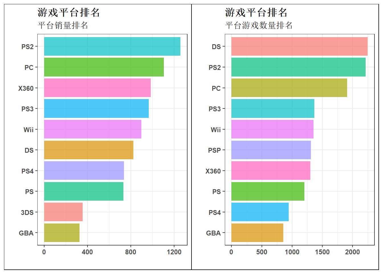
1.3.1.2 游戏平台排名（销量、游戏数量）

df_platform <- df %>% 
  select(Platform, Total_Shipped) %>% 
  group_by(Platform) %>% 
  summarize(amount = sum(Total_Shipped)) %>% 
  arrange(desc(amount)) %>% 
  head(10)

p3 <- ggplot(df_platform, aes(x = reorder(Platform, amount), y = amount, 
                                    fill = Platform)) +
  geom_bar(stat = "identity", alpha = 0.7) +
  labs(x = " ", y = " ") +
  ggtitle("游戏平台排名", subtitle = "平台销量排名") +
  coord_flip() +
  theme_bw() +
  theme(legend.position = "none",
        axis.text = element_text(face = "bold"), 
        plot.title = element_text(face = "bold"),
        plot.background = element_rect(color = "black"))

df_platform2 <- as.data.frame(table(df$Platform)) %>% 
  rename(Platform = Var1) %>% 
  arrange(desc(Freq)) %>% 
  head(10)

p4 <- ggplot(df_platform2, aes(x = reorder(Platform, Freq), y = Freq, 
                         fill = Platform)) +
  geom_bar(stat = "identity", alpha = 0.7) +
  labs(x = " ", y = " ") +
  ggtitle("游戏平台排名", subtitle = "平台游戏数量排名") +
  coord_flip() +
  theme_bw() +
  theme(plot.background = element_rect(color = "black"), 
        legend.position = "none",
        plot.title = element_text(face = "bold"),
        axis.text = element_text(face = "bold"))
p3|p4

由图@ref(fig:platform)可以看出：

PS2不愧是有史以来最成功的的家用主机，发行在其上的游戏销量排名第一、游戏数量排名第二。
PC游戏仍有一定竞争力。
御三家统治了主机游戏。

下面我们看一下游戏开发商的情况。

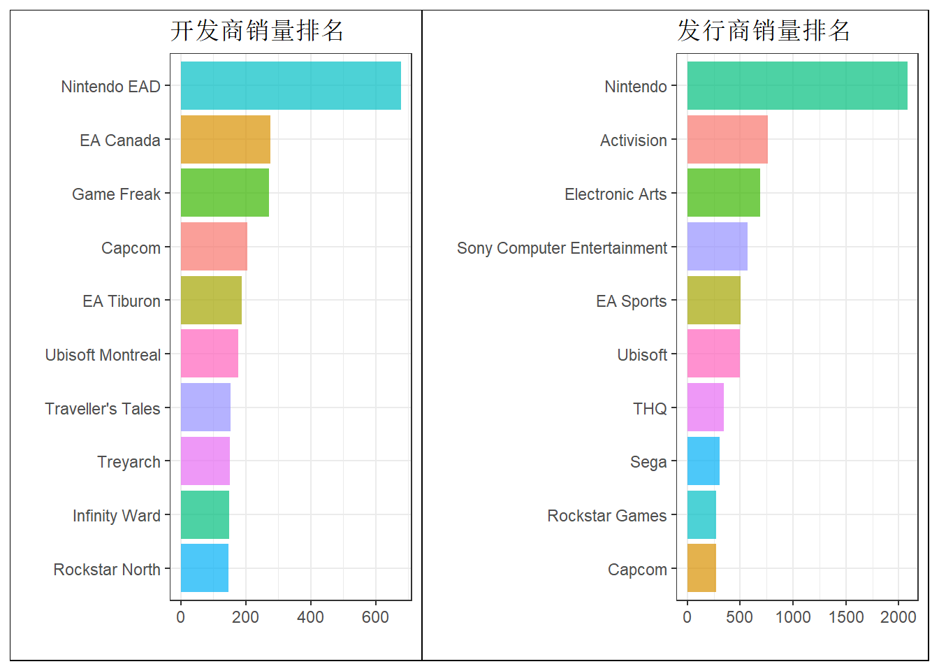
1.3.1.3 开发商和发行商排名

df_developer <-  df %>% 
  select(Developer, Total_Shipped) %>% 
  group_by(Developer) %>% 
  summarise(amount = sum(Total_Shipped)) %>% 
  arrange(desc(amount)) %>% 
  head(10)

p5 <- ggplot(df_developer, aes(x = reorder(Developer, amount), y = amount,
                         fill = Developer)) +
  geom_bar(stat = "identity", alpha = 0.7) +
  coord_flip() +
  ggtitle("开发商销量排名") +
  labs(x = " ", y = "") +
  theme_bw() +
  theme(legend.position = "none",
        plot.background = element_rect(color = "black"))

df_publisher <- df %>% 
  select(Publisher, Total_Shipped) %>% 
  group_by(Publisher) %>% 
  summarise(amount = sum(Total_Shipped)) %>% 
  arrange(desc(amount)) %>% 
  head(10)

p6 <- ggplot(df_publisher, aes(x = reorder(Publisher, amount), y = amount,
                         fill = Publisher)) +
  geom_bar(stat = "identity", alpha = 0.7) +
  coord_flip() +
  ggtitle("发行商销量排名") +
  labs(x = " ", y = "") +
  theme_bw() +
  theme(legend.position = "none",
        plot.background = element_rect(color = "black"))
p5|p6

任天堂作为开发商和发行商均独占鳌头。
Game Freak依靠王牌IP精灵宝可梦占据开发商销量第三名。
大家耳熟能详的游戏开发商和发行商均有上榜。

1.4 探索性分析

在统计学中，探索性数据分析 (EAD) 是一种分析数据集以总结其主要特征的方法，通常使用可视化方法。

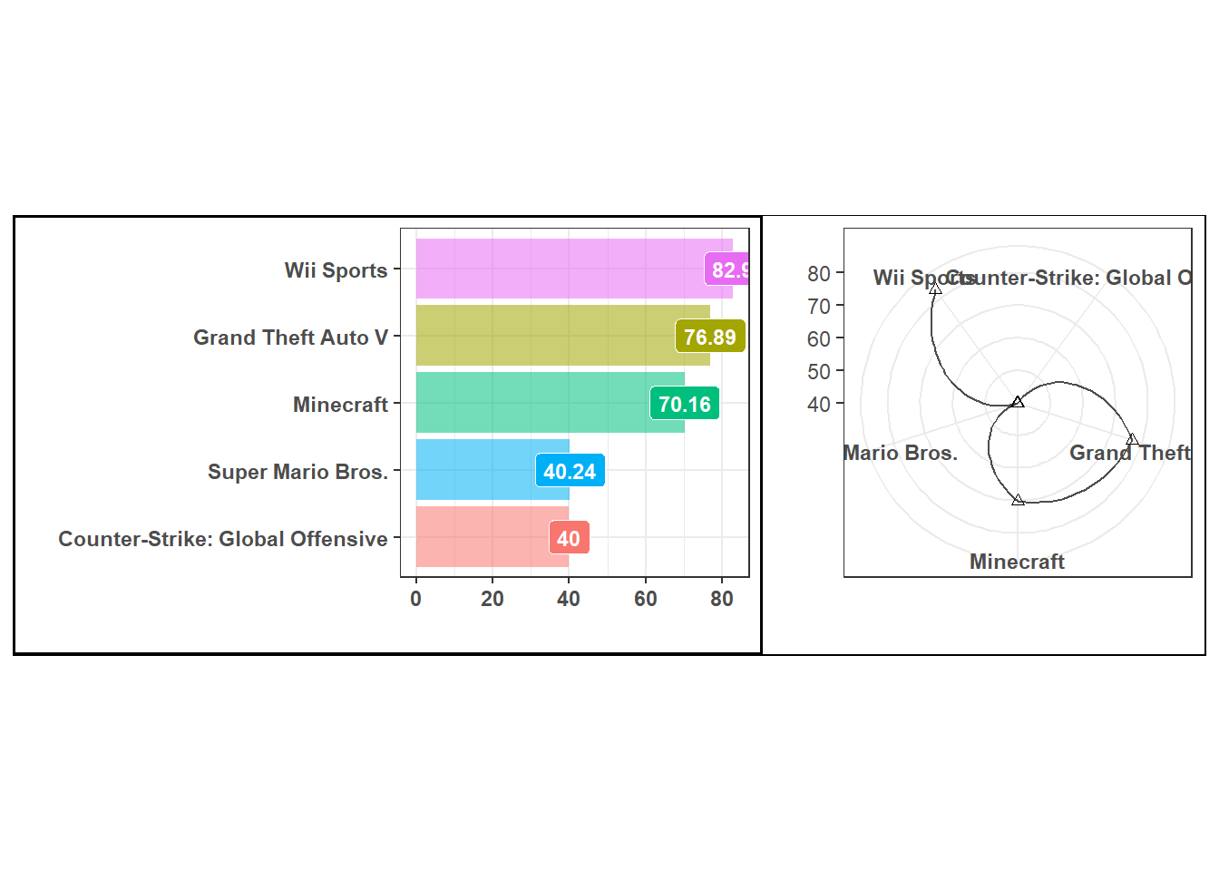
1.4.1 世界最畅销游戏

1.4.1.1 最畅销的5个游戏

那么，1977年~2019年间，到底哪个游戏销量是最高的呢？

options(repr.plot.width = 20, repr.plot.height = 8)

df_games <- df %>% 
  select(Name, Total_Shipped) %>% 
  group_by(Name) %>% 
  summarise(amount = sum(Total_Shipped)) %>% 
  arrange(desc(amount)) %>% 
  head(5)

p7 <- ggplot(df_games, aes(x = reorder(Name, amount), y = amount,
                     fill = Name)) +
  geom_col(aes(alpha = 0.9)) +
  geom_label(aes(label = amount), size = 3,
             fontface = "bold",
             color = "white") +
  labs(x = " ", y = " ") +
  coord_flip() +
  theme_bw() +
  theme(legend.position = "none",
        plot.background = element_rect(color = "black", size = 1.1),
        axis.text.x = element_text( face = "bold"),
        axis.text.y = element_text(face = "bold"))

p8 <- ggplot(df_games, aes(x = Name, y = amount)) +
  geom_line(alpha = 0.7, group = 1) +
  geom_point(aes(fill = Name), shape = 2) +
  theme_bw()+ 
  theme(legend.position = "none",
        plot.background = element_rect(color = "black"),
        axis.text.x = element_text(face = "bold")) +
  labs(x = "", y = "") +
  coord_polar()
p7|p8

由图@ref(fig:games)可知：

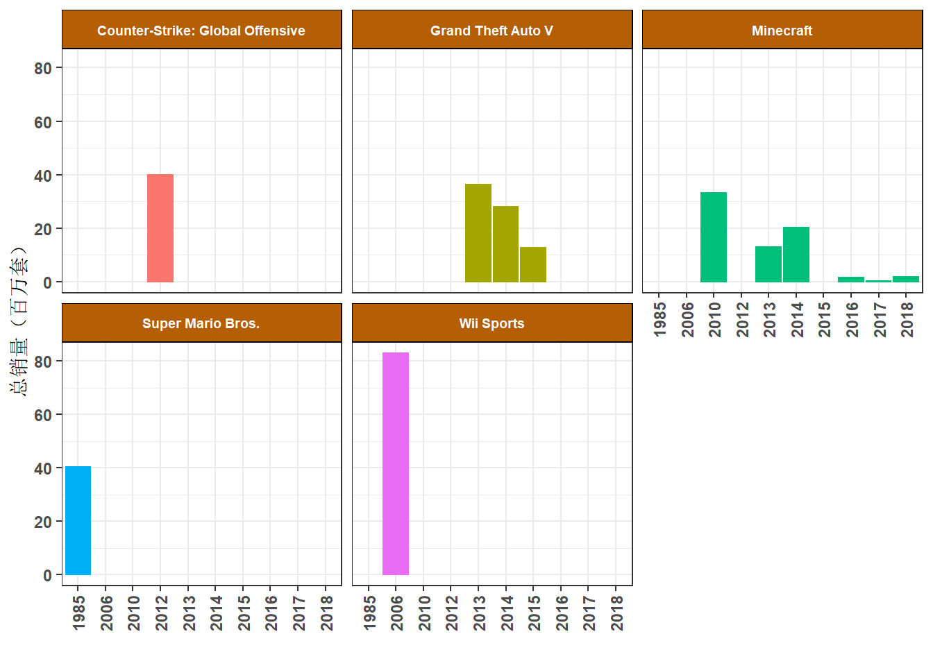
游戏销量排名前3的游戏为：Wii Sports、GTA5和我的世界。
GTV5和我的世界在多个游戏平台均有发售，Wii Sports为任天堂平台独占。
任天堂游戏平台发售的游戏占前十的大多数，任天堂就是世界的主宰！

1.4.1.2 最畅销的5个游戏逐年分布

df_games_top5 <- df %>% 
  filter(Name == "Wii Sports" |
         Name == "Grand Theft Auto V"|
         Name == "Minecraft"|
         Name == "Super Mario Bros."|
         Name == "Counter-Strike: Global Offensive") %>% 
  select(Name, Year, Total_Shipped)

ggplot(df_games_top5, aes(x = Year, y = Total_Shipped)) +
  geom_bar(stat = "identity", aes(fill = Name, 
                                  color = Name),
           alpha = 8) +
  facet_wrap(~Name) +
  labs(x = "", y = "总销量（百万套）") +
  theme_bw()+
  theme(legend.position = "none",
        strip.text.x = element_text(
          margin = margin(7, 7, 7, 7), size = 7, 
          face = "bold", color = "white"),
        strip.background = element_rect(fill = "#B45F04",
                                        color = "black"),
        plot.title = element_text(face = "bold"),
        axis.text.x = element_text(face = "bold",
                                   angle = 90,
                                   vjust = 0.5),
        axis.text.y = element_text(face = "bold"))

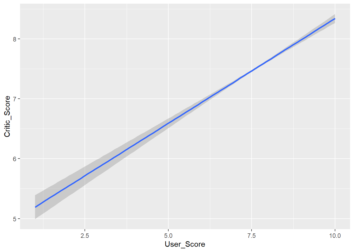
1.5 媒体打分与玩家打分的关系

俗话说，“低分信媒体，高分信自己”。如果一款游戏媒体打分低，那肯定不行，但如果一个游戏媒体打高分，也不一定好玩（有可能是塞了钱）。

下面我们就分析一下媒体打分与玩家打分的关系。

df_score <- df %>% 
  select(Name, User_Score, Critic_Score) 

cor <- cor.test(df_score$User_Score, df_score$Critic_Score,
                method = "pearson")
p.value  <-  cor$p.value
coef  <- cor$estimate 

ggplot(df_score, aes(x = User_Score, y = Critic_Score)) +
  geom_smooth(method = lm)

可以看到两个打分的相关系数为0.16，且p值小于0.05，表明两者呈现显著的正相关。看来游戏媒体和玩家对游戏的口味还是一样的，某种程度上说，高分也可以信媒体。

1.6 玩家与媒体分别最喜欢哪个发行商

1.6.1 玩家

那么，玩家最喜欢（打分最高）的游戏发行商是谁呢？

df_player <- df %>% 
  select(Publisher, User_Score)

df_player$Publisher <- df_player$Publisher %>% 
  map(~
        str_detect(.x,"Sony") %>% 
        ifelse("Sony", .x)) %>% 
  unlist() 

df_player <- df_player%>% 
  group_by(Publisher) %>% 
  summarise(count = n(),
            mean_score = mean(User_Score)) %>% 
  filter(count >= 50) %>% 
  select(Publisher, mean_score) %>% 
  arrange(desc(mean_score))
df_player

# A tibble: 62 × 2
   Publisher                mean_score
   <chr>                         <dbl>
 1 Rockstar Games                 7.84
 2 Microsoft Game Studios         7.77
 3 Nintendo                       7.77
 4 Sierra Entertainment           7.72
 5 DreamCatcher Interactive       7.71
 6 5pb                            7.71
 7 Sony                           7.70
 8 Eidos Interactive              7.70
 9 Acclaim Entertainment          7.7 
10 Agetec                         7.7 
# … with 52 more rows

在发行过50个以上游戏的老牌发行商中：

R星凭借GTA、荒野大镖客等重量级IP以7.842的评分独占鳌头。
所有发行商的评分均超过7分，说明现代游戏的质量还是有保障的。