5  学生成绩水平分类

5.1 数据变量说明

变量说明。

变量中最重要的的为Class学生等级变量，是我们建模的目标变量。

edudata <- read_csv("data/xAPI-Edu-Data.csv")
edudata$Class <- factor(edudata$Class, levels = c("H", "M", "L"))
edudata$gender <- factor(edudata$gender, levels = c("M", "F"))
str(edudata)

spec_tbl_df [480 × 17] (S3: spec_tbl_df/tbl_df/tbl/data.frame)
 $ gender                  : Factor w/ 2 levels "M","F": 1 1 1 1 1 2 1 1 2 2 ...
 $ NationalITy             : chr [1:480] "KW" "KW" "KW" "KW" ...
 $ PlaceofBirth            : chr [1:480] "KuwaIT" "KuwaIT" "KuwaIT" "KuwaIT" ...
 $ StageID                 : chr [1:480] "lowerlevel" "lowerlevel" "lowerlevel" "lowerlevel" ...
 $ GradeID                 : chr [1:480] "G-04" "G-04" "G-04" "G-04" ...
 $ SectionID               : chr [1:480] "A" "A" "A" "A" ...
 $ Topic                   : chr [1:480] "IT" "IT" "IT" "IT" ...
 $ Semester                : chr [1:480] "F" "F" "F" "F" ...
 $ Relation                : chr [1:480] "Father" "Father" "Father" "Father" ...
 $ raisedhands             : num [1:480] 15 20 10 30 40 42 35 50 12 70 ...
 $ VisITedResources        : num [1:480] 16 20 7 25 50 30 12 10 21 80 ...
 $ AnnouncementsView       : num [1:480] 2 3 0 5 12 13 0 15 16 25 ...
 $ Discussion              : num [1:480] 20 25 30 35 50 70 17 22 50 70 ...
 $ ParentAnsweringSurvey   : chr [1:480] "Yes" "Yes" "No" "No" ...
 $ ParentschoolSatisfaction: chr [1:480] "Good" "Good" "Bad" "Bad" ...
 $ StudentAbsenceDays      : chr [1:480] "Under-7" "Under-7" "Above-7" "Above-7" ...
 $ Class                   : Factor w/ 3 levels "H","M","L": 2 2 3 3 2 2 3 2 2 2 ...
 - attr(*, "spec")=
  .. cols(
  ..   gender = col_character(),
  ..   NationalITy = col_character(),
  ..   PlaceofBirth = col_character(),
  ..   StageID = col_character(),
  ..   GradeID = col_character(),
  ..   SectionID = col_character(),
  ..   Topic = col_character(),
  ..   Semester = col_character(),
  ..   Relation = col_character(),
  ..   raisedhands = col_double(),
  ..   VisITedResources = col_double(),
  ..   AnnouncementsView = col_double(),
  ..   Discussion = col_double(),
  ..   ParentAnsweringSurvey = col_character(),
  ..   ParentschoolSatisfaction = col_character(),
  ..   StudentAbsenceDays = col_character(),
  ..   Class = col_character()
  .. )
 - attr(*, "problems")=<externalptr> 

5.2 描述性分析

5.2.1 封装绘图函数

fun_bar <- function(data, xlab, fillc, pos, xname, yname, legend){
  data %>% 
    group_by({{xlab}}) %>% # dplyr中的自定函数参数需要使用{{}}括起来
    mutate(count = n()) %>% 
      ggplot(aes(reorder({{xlab}}, count), count, fill = {{fillc}})) +
      geom_col(position = pos) + #pos = "stack" or "fill"
      labs(x = xname, y = yname) +
      coord_flip() +
      theme_bw() +
      guides(fill = guide_legend(title = legend))
}

5.2.2 不同教育程度的学生选择课程主题

p1 <- fun_bar(data = edudata, xlab = Topic, fillc = StageID,
             pos = "stack", xname = "Topic", yname = "Student_Count",
             legend = "教育程度")
p2 <- fun_bar(data = edudata, xlab = Topic, fillc = StageID,
             pos = "fill", xname = "Topic", yname = "Per_Student_Count",
             legend = "教育程度")
p1/p2

不同教育程度的学生选择课程主题

由图@ref(fig:school-level)可以看出：

• 课程主题最多的为IT、French和Arabic，其中选择IT的课程主题的学员远高于其他课。

• 无论哪种教育程度，IT、Science、Math和English四种课程都是必修的（三种颜色都有）。

5.2.3 不同课程主题监护人情况

这部分主要针对家长的情况进行分析，了解父母对学员学习的不同情况。对应在数据集中的变量为Relation。

p3 <- fun_bar(data = edudata, xlab = Topic, fillc = Relation,
              pos = "stack", xname = "Topic", yname = "Student_count",
              legend = "监护人情况")
p4 <- fun_bar(data = edudata, xlab = Topic, fillc = Relation,
              pos = "fill", xname = "Topic", yname = "Student_count",
              legend = "监护人情况")
p3/p4

不同课程主题监护人情况

由图@ref(fig:relation)可以看出：

• 总体而言，监护人为父亲的较多。其中，IT和Math课程中，负责人为父亲的超过75%。

• French课程，监护人大多数为母亲，占70%左右。

5.2.4 不同课程学生学习成绩

p5 <- fun_bar(data = edudata, xlab = Topic, fillc = Class,
              pos = "stack", xname = "Topic", yname = "Student_count",
              legend = "学生成绩")
p6 <- fun_bar(data = edudata, xlab = Topic, fillc = Class,
              pos = "fill", xname = "Topic", yname = "Student_count",
              legend = "学生成绩")
p5/p6

不同课程学生学习成绩

由图@ref(fig:class):

• 所有课程中，只有Biology课程中，属于高水平的学生数超过了50%。

• 在Geology课程中，没有低水平的学生。

5.2.5 不同教室学生成绩水平

p7 <- fun_bar(data = edudata, xlab = SectionID, fillc = Class,
              pos = "stack", xname = "Section_ID", yname = "Student_count",
              legend = "学生成绩")
p8 <- fun_bar(data = edudata, xlab = SectionID, fillc = Class,
              pos = "fill", xname = "Section_ID", yname = "Student_count",
              legend = "学生成绩")
p7/p8

不同教室学生成绩水平

由图@ref(fig:score-section)可以看出：

• 在A班的学生最多，C班的学生最少。

• C班的低水平成绩的学生相对较多，其它两个班级的成绩水平基本一致。

5.2.6 不同学期、不同成绩水平与监护人的关系

# 封装函数，去掉坐标轴翻转
fun_bar2 <- function(data, xlab, fillc, pos, xname, yname, legend){
  data %>% 
    group_by({{xlab}}) %>% # dplyr中的自定函数参数需要使用{{}}括起来
    mutate(count = n()) %>% 
      ggplot(aes(reorder({{xlab}}, count), count, fill = {{fillc}})) +
      geom_col(position = pos) + #pos = "stack" or "fill"
      labs(x = xname, y = yname) +
      theme_bw() +
      guides(fill = guide_legend(title = legend))
}

p9 <- fun_bar2(edudata, Semester, Relation, pos = "stack",
              xname = "Semester", yname = "Student_count",
              legend = "监护人情况")

p10 <- fun_bar2(edudata, Semester, Relation, pos = "fill",
              xname = "Semester", yname = "per_Student_count",
              legend = "监护人情况")

p11 <- fun_bar2(edudata, Class, Relation, pos = "stack",
               xname = "Class", yname = "Student_count",
               legend = "监护人情况")

p12 <- fun_bar2(edudata, Class, Relation, pos = "fill",
               xname = "Class", yname = "per_Student_count",
               legend = "监护人情况")
(p9|p10) / (p11|p12)

不同学期、不同成绩水平与监护人的关系

由图@ref(fig:semester)可知：

• 第一学期父亲作为监护人的学生数比第二学期多。

• 总体看，成绩水平较高的学生中，监护人为母亲的比较多；其它水平均是父亲较多。

5.2.7 家长是否回答调查问卷、成绩水平与家长对学校是否满意的关系

p13 <- fun_bar2(edudata, ParentAnsweringSurvey, ParentschoolSatisfaction, 
                pos = "stack", xname = "ParentAnsweringSurvey",
                yname = "Student_count", legend = "是否满意")
p14 <- fun_bar2(edudata, ParentAnsweringSurvey, ParentschoolSatisfaction, 
                pos = "fill", xname = "ParentAnsweringSurvey",
                yname = "Per_Student_count", legend = "是否满意")

p15 <- fun_bar2(edudata, Class, ParentschoolSatisfaction, 
                pos = "stack", xname = "Class",
                yname = "Student_count", legend = "是否满意")
p16 <- fun_bar2(edudata, Class, ParentschoolSatisfaction, 
                pos = "fill", xname = "Class",
                yname = "Per_Student_count", legend = "是否满意")
(p13|p14)/(p15|p16)

家长是否回答调查问卷、成绩水平与家长对学校是否满意的关系

由图@ref(fig:surey-class)可以看出：

• 有超过一半的家长回答了问卷，其中，回答问卷的家长大部分对学校满意，而未回答问卷的则大部分对学校不满。

• 成绩越高，家长对学校越满意。

5.2.8 性别、逃课次数与学生成绩水平的关系

p17 <- fun_bar2(edudata, gender, Class, 
                pos = "stack", xname = "Gender",
                yname = "Student_count", legend = "成绩水平")
p18 <- fun_bar2(edudata, gender, Class, 
                pos = "fill", xname = "Gender",
                yname = "Per_Student_count", legend = "成绩水平")

p19 <- fun_bar2(edudata, StudentAbsenceDays, Class, 
                pos = "stack", xname = "Class",
                yname = "Student_count", legend = "成绩水平")
p20 <- fun_bar2(edudata, StudentAbsenceDays, Class, 
                pos = "fill", xname = "Class",
                yname = "Per_Student_count", legend = "成绩水平")
(p17|p18)/(p19|p20)

性别、逃课次数与学生成绩水平的关系

由图@ref(fig:gender-absence)可知：

• 女生比男生数量少很多，但高水平成绩的人数明显比男生多；中水平成绩男女比例基本持平。

• 逃课超过7天的的学生基本无法取得好的成绩。

5.2.9 举手次数和参加讨论次数与成绩水平关系

fun_bar3 <- function(data, xlab, ylab, fillc, xname, yname){
  data %>% 
    group_by({{xlab}}) %>% 
    summarise(Mcount = mean({{ylab}})) %>% 
     ggplot(aes({{xlab}}, Mcount, fill = {{fillc}})) +
      geom_col() + 
      labs(x = xname, y = yname) +
      theme_bw() +
      theme(legend.position = "none")
}

# edudata$Class <- factor(edudata$Class, c("H", "M", "L"), ordered = TRUE)
p21 <- fun_bar3(data = edudata, xlab = Class, ylab = raisedhands, 
                fillc = Class, "成绩水平", "平均举手次数" )

p22 <- fun_bar3(data = edudata, xlab = Class, ylab = Discussion, 
                fillc = Class, "成绩水平", "平均参与讨论次数" )
p21|p22

举手次数和参加讨论次数与成绩水平关系

由图@ref(fig:raisedhands-discuss)可知： 举手次数和参与讨论次数越多，成绩水平越高。

---

5.3 模型建立

5.3.1 回归树模型建立

set.seed(1234)
# 按照数据目标8:2进行分层抽样，返回矩阵形式的抽样索引
index <- createDataPartition(edudata$Class, p = 0.8, list = F)
train <- edudata[index, ]
test <- edudata[-index, ]

# 建立回归树模型
rpart_model <- rpart(Class ~., data = train)
# type = "class"指定预测结果是具体的某个类别
pred_rp <- predict(rpart_model, test[-17], type = "class")
confusionMatrix(pred_rp, test$Class)

Confusion Matrix and Statistics

          Reference
Prediction  H  M  L
         H 18  3  0
         M  9 29  3
         L  1 10 22

Overall Statistics
                                          
               Accuracy : 0.7263          
                 95% CI : (0.6252, 0.8128)
    No Information Rate : 0.4421          
    P-Value [Acc > NIR] : 1.882e-08       
                                          
                  Kappa : 0.5806          
                                          
 Mcnemar's Test P-Value : 0.05103         

Statistics by Class:

                     Class: H Class: M Class: L
Sensitivity            0.6429   0.6905   0.8800
Specificity            0.9552   0.7736   0.8429
Pos Pred Value         0.8571   0.7073   0.6667
Neg Pred Value         0.8649   0.7593   0.9516
Prevalence             0.2947   0.4421   0.2632
Detection Rate         0.1895   0.3053   0.2316
Detection Prevalence   0.2211   0.4316   0.3474
Balanced Accuracy      0.7990   0.7320   0.8614

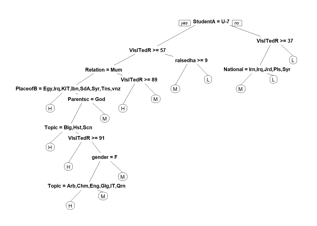
prp(rpart_model)

5.3.2 随机数模型

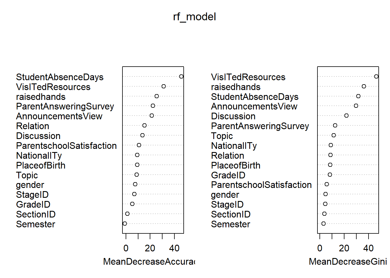
set.seed(1234)
# importance = T:稍后对变量进行重要性的可视化
rf_model <- randomForest(Class~., data = train, importance = T)
pred_rf <- predict(rf_model, test[-17], type = "class")
confusionMatrix(pred_rf, test$Class) # 混淆矩阵判断模型准确率

Confusion Matrix and Statistics

          Reference
Prediction  H  M  L
         H 20  4  0
         M  8 36  4
         L  0  2 21

Overall Statistics
                                          
               Accuracy : 0.8105          
                 95% CI : (0.7172, 0.8837)
    No Information Rate : 0.4421          
    P-Value [Acc > NIR] : 1.886e-13       
                                          
                  Kappa : 0.7032          
                                          
 Mcnemar's Test P-Value : NA              

Statistics by Class:

                     Class: H Class: M Class: L
Sensitivity            0.7143   0.8571   0.8400
Specificity            0.9403   0.7736   0.9714
Pos Pred Value         0.8333   0.7500   0.9130
Neg Pred Value         0.8873   0.8723   0.9444
Prevalence             0.2947   0.4421   0.2632
Detection Rate         0.2105   0.3789   0.2211
Detection Prevalence   0.2526   0.5053   0.2421
Balanced Accuracy      0.8273   0.8154   0.9057

varImpPlot(rf_model) # 可视化变量重要性函数

阅读上图：

• 圆点越靠近右侧越重要。

• 我们重点观察排名前五的变量。通过左右两图的对比发现，两图中前四个变量相同（交叉），可以判定这四个变量是数据中最重要的变量。

5.3.3 SVM建模-支持向量机(需要再研究)

set.seed(1234)
library(kernlab) # Kernel-Based Machine Learning Lab
svm_model <- ksvm(Class~., data = test, kernel = "rbfdot")
# type = "response":指定预测结果是具体的某个列别
pred_svm <- predict(svm_model, test[-17], type = "response")
confusionMatrix(pred_svm, test$Class)

Confusion Matrix and Statistics

          Reference
Prediction  H  M  L
         H 23  4  0
         M  5 36  1
         L  0  2 24

Overall Statistics
                                         
               Accuracy : 0.8737         
                 95% CI : (0.7897, 0.933)
    No Information Rate : 0.4421         
    P-Value [Acc > NIR] : < 2.2e-16      
                                         
                  Kappa : 0.8053         
                                         
 Mcnemar's Test P-Value : NA             

Statistics by Class:

                     Class: H Class: M Class: L
Sensitivity            0.8214   0.8571   0.9600
Specificity            0.9403   0.8868   0.9714
Pos Pred Value         0.8519   0.8571   0.9231
Neg Pred Value         0.9265   0.8868   0.9855
Prevalence             0.2947   0.4421   0.2632
Detection Rate         0.2421   0.3789   0.2526
Detection Prevalence   0.2842   0.4421   0.2737
Balanced Accuracy      0.8809   0.8720   0.9657

5.3.4 模型融合

将各个模型的结果做一个融合（合并至一个数据框）。

result <- data.frame(rpart = pred_rp,
                     randomForest = pred_rf,
                     svm = pred_svm,
                     actual_class = test$Class, 
                     final_pred = rep("-", nrow(test)))
head(result)

  rpart randomForest svm actual_class final_pred
1     M            M   M            M          -
2     L            L   L            L          -
3     L            L   L            L          -
4     M            M   L            M          -
5     L            L   L            L          -
6     M            M   M            M          -

# 封装求众数函数
fun_pred <- function(x){
  names(which.max(table(x)))
}

result$final_pred <- factor(apply(result[1:2], 1, fun_pred))
confusionMatrix(result$actual_class, result$final_pred)

Confusion Matrix and Statistics

          Reference
Prediction  H  L  M
         H 21  1  6
         L  0 23  2
         M  7 10 25

Overall Statistics
                                          
               Accuracy : 0.7263          
                 95% CI : (0.6252, 0.8128)
    No Information Rate : 0.3579          
    P-Value [Acc > NIR] : 3.029e-13       
                                          
                  Kappa : 0.5887          
                                          
 Mcnemar's Test P-Value : 0.09327         

Statistics by Class:

                     Class: H Class: L Class: M
Sensitivity            0.7500   0.6765   0.7576
Specificity            0.8955   0.9672   0.7258
Pos Pred Value         0.7500   0.9200   0.5952
Neg Pred Value         0.8955   0.8429   0.8491
Prevalence             0.2947   0.3579   0.3474
Detection Rate         0.2211   0.2421   0.2632
Detection Prevalence   0.2947   0.2632   0.4421
Balanced Accuracy      0.8228   0.8218   0.7417

head(result)

  rpart randomForest svm actual_class final_pred
1     M            M   M            M          M
2     L            L   L            L          L
3     L            L   L            L          L
4     M            M   L            M          M
5     L            L   L            L          L
6     M            M   M            M          M