描述性分析
数据概览
<- read.csv ("data/HR_comma_sep.csv" )summary (hr)
 satisfaction_level last_evaluation  number_project  average_montly_hours
 Min.   :0.0900     Min.   :0.3600   Min.   :2.000   Min.   : 96.0
 1st Qu.:0.4400     1st Qu.:0.5600   1st Qu.:3.000   1st Qu.:156.0
 Median :0.6400     Median :0.7200   Median :4.000   Median :200.0
 Mean   :0.6128     Mean   :0.7161   Mean   :3.803   Mean   :201.1
 3rd Qu.:0.8200     3rd Qu.:0.8700   3rd Qu.:5.000   3rd Qu.:245.0
 Max.   :1.0000     Max.   :1.0000   Max.   :7.000   Max.   :310.0
 time_spend_company Work_accident         left        promotion_last_5years
 Min.   : 2.000     Min.   :0.0000   Min.   :0.0000   Min.   :0.00000
 1st Qu.: 3.000     1st Qu.:0.0000   1st Qu.:0.0000   1st Qu.:0.00000
 Median : 3.000     Median :0.0000   Median :0.0000   Median :0.00000
 Mean   : 3.498     Mean   :0.1446   Mean   :0.2381   Mean   :0.02127
 3rd Qu.: 4.000     3rd Qu.:0.0000   3rd Qu.:0.0000   3rd Qu.:0.00000
 Max.   :10.000     Max.   :1.0000   Max.   :1.0000   Max.   :1.00000
    sales              salary
 Length:14999       Length:14999
 Class :character   Class :character
 Mode  :character   Mode  :character
观察各个变量的主要描述统计量,可知:
离职率(left)平均将近24%。
对公司的满意度(satisfaction_level)仅有62%左右。
平均每个人参加过的项目数(number_project)仅为3~4个。
员工每月平均工作时间(average_montly_hours)达到201.1小时,按照每月工作20天(去除8天双休)计算,每个员工平均每天工作超过10小时。
员工离职情况与员工满意度、月均工作时间、绩效评估和在职年限的关系
我们通过绘图观察离职员工的特点。
$ left <- factor (hr$ left, levels = c ("0" , "1" ))# 离职率与公司满意度关系 <- ggplot (hr, aes (x = left, y = satisfaction_level,fill = left)) + geom_boxplot () + theme_bw () + labs (x = "离职情况" , y = "员工满意度" ) + guides (fill = guide_legend (title = "离职情况" ))# 离职率与绩效评估的关系 <- ggplot (hr, aes (x = left, y = last_evaluation,fill = left)) + geom_boxplot () + theme_bw () + labs (x = "离职情况" , y = "绩效评估" ) + guides (fill = guide_legend (title = "离职情况" ))# 离职率与月均工作时间的关系 <- ggplot (hr, aes (x = left, y = average_montly_hours, fill = left)) + geom_boxplot () + theme_bw ()+ labs (x = "离职率" , y = "月均工作时间" ) + guides (fill = guide_legend (title = "离职情况" ))# 离职率与工作年限的关系 <- ggplot (hr, aes (x = left, y = time_spend_company, fill = left)) + geom_boxplot () + theme_bw () + labs (x = "离职率" , y = "在职年限" ) + guides (fill = guide_legend (title = "离职情况" ))/ boxEva | boxMonth/ boxTime
(ref:fig-resigned) 员工离职情况与员工满意度、月均工作时间、绩效评估和在职年限的关系。
由图@ref(fig:boxplot-resigned)可以看出,离职员工的几个特点:
左上图:离职员工的满意度明显低于未离职的满意度,大都集中于0.4左右。
左下图:离职员工的绩效评估较高。推测离职员工倾向于寻找待遇更好的工作。
右上图:离职员工的月均工作时长较高,大部分超过了平均水平(200小时)。
右下图:工作年限均在4年左右。
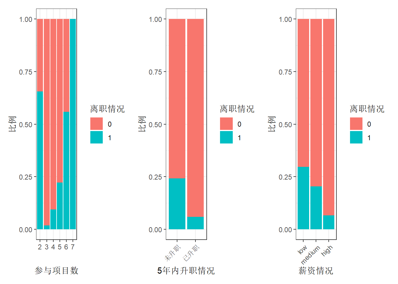
员工离职情况与项目参与个数、五年内升职情况和薪资的关系
$ number_project <- factor (hr$ number_project,levels = c ("2" , "3" , "4" , "5" , "6" , "7" ))# 离职与参与项目数关系 <- ggplot (hr, aes (x = number_project, fill = left)) + geom_bar (position = "fill" ) + # fill为百分比条形图 theme_bw () + labs (x = "参与项目数" , y = "比例" ) + guides (fill = guide_legend (title = "离职情况" ))# 离职与升职情况关系 $ promotion_last_5years[hr$ promotion_last_5years == 1 ] <- "已升职" $ promotion_last_5years[hr$ promotion_last_5years == 0 ] <- "未升职" <- ggplot (hr, aes (x = as.factor (promotion_last_5years), fill = left)) + geom_bar (position = "fill" ) + theme_bw () + labs (x = "5年内升职情况" , y = "比例" ) + theme (axis.text.x = element_text (angle = 45 ,hjust = 1 )) + guides (fill = guide_legend (title = "离职情况" ))# 离职与薪资关系 <- ggplot (hr, aes (x = factor (salary, levels = c ("low" , "medium" , "high" ), ordered= TRUE ), fill = left)) + geom_bar (position = "fill" ) + theme_bw () + labs (x = "薪资情况" , y = "比例" ) + theme (axis.text.x = element_text (angle = 45 ,hjust = 1 )) + guides (fill = guide_legend (title = "离职情况" )) | bar5years | barSalary
(ref:fig-bar-resigned) 员工离职情况与项目参与个数、五年内升职情况和薪资的关系。
由图@ref(fig:barplot-resigned)可以看出,离职员工的几个特点:
参与项目过少(2个)与过多(7个)的员工离职率均比较高。且参与项目在3个及以上时,参与项目越多,离职率越高。
5年内未升职的员工离职率较高。
薪资越低,离职率越高。
建模预测1-回归树+混淆矩阵
建模的思路:
提取所需数据。
定义交叉验证方法。
进行分层抽样,提取出想要的训练集和测试集。
实际建模。
对数据进行预测(利用混淆矩阵的方式)。
提取数据
选择符合条件的样本。通过绩效评估、在职时间和参与项目数筛选出更有代表性的样本数据进行分析。 按照绩效评估、在职时间、参与项目数量
<- hr %>% filter (last_evaluation >= 0.70 | >= 4 | >= 5 )
确定交叉验证方法
# cv为设置交叉验证方法,number = 5为5折交叉验证。 <- trainControl (method = "cv" ,number = 5 )
分层抽样
# 设定随机种子,确保每次抽样结果一致。 set.seed (1234 )# 根据数据因变量进行7:3的分层抽样,返回行索引向量 p = 0.7为按照7:3进行抽样 # 参数list表示返回值是否为列表 <- createDataPartition (hr_model$ left,p = 0.7 , list = F)# 以index为索引的数据为训练集 # 剩余的数据为测试集 <- hr_model[index, ]<- hr_model[- index, ]
实际建模
使用carte包中的train函数对训练集进行5折交叉验证建立回归树模型。
# left~. 代表因变量left与所有自变量进行建模。 <- train (left~ ., data = trainData,trControl = train_control,method = "rpart" )
利用建立好的模型rpartmodel对测试集进行预测。
# testdata[-7]剔除left列。 <- predict (rpartmodel, testData[- 7 ])
建立混淆矩阵,验证建立的模型。
<- table (predRpart, testData$ left)
predRpart    0    1
        0 2246   72
        1   51  528
混淆矩阵:混淆矩阵的每一列代表了预测类别,每一列的总数表示预测为该类别的数据的数目;每一行代表了数据的真实归属类别,每一行的数据总数表示该类别的数据实例的数目。根据查全率和查准率两个参数判断模型拟合结果是否够好。
混淆矩阵的查准率和查全率是两个重要的参数,具体计算公式如下式@ref(eq:three-CM):
\[\begin{align}
查准率=\frac{真正例}{真正例+假正例} \\
查全率=\frac{真正例}{真正例+假反例}
(\#eq:three-CM)
\end{align}\]
根据混淆矩阵结果,可以得到回归树模型的:
查准率为91.19 %。
查全率为88 %。
回归模型的拟合效果不错。
建模预测2-朴素贝叶斯
建模步骤与第@ref(sec:three-model1)小结基本相同,下面只列出代码及结果。
<- train (left~ ., data = trainData,trControl = train_control,method = "nb" )<- predict (nbModel, testData[- 7 ])<- table (predNb, testData$ left)
predNb    0    1
     0 2248  146
     1   49  454
根据公式@ref(eq:three-CM),计算得到朴素贝叶斯模型的:
查准率为90.26 %。
查全率为75.67 %。
通过两种模型的评估,我们发现回归树模型的拟合度比朴素贝叶斯更好,所以接下来我们采用回归数模型进行进一步分析。
模型评估及应用
ROC曲线绘制
绘制ROC曲线的数据必须是数值型。
<- as.numeric (as.character (predRpart))<- as.numeric (predNb)
转换后绘制图形。
# 获取后续绘图使用的信息 <- roc (testData$ left, predRpart)# 计算两个关键值 # 假正例率 <- rocPart$ specificities# 查全率,即真正利率 <- rocPart$ sensitivities
# 获取后续绘图使用的信息 <- roc (testData$ left, predNb)# 计算两个关键值 # 假正例率 <- rocNb$ specificities# 查全率,即真正利率 <- rocNb$ sensitivities
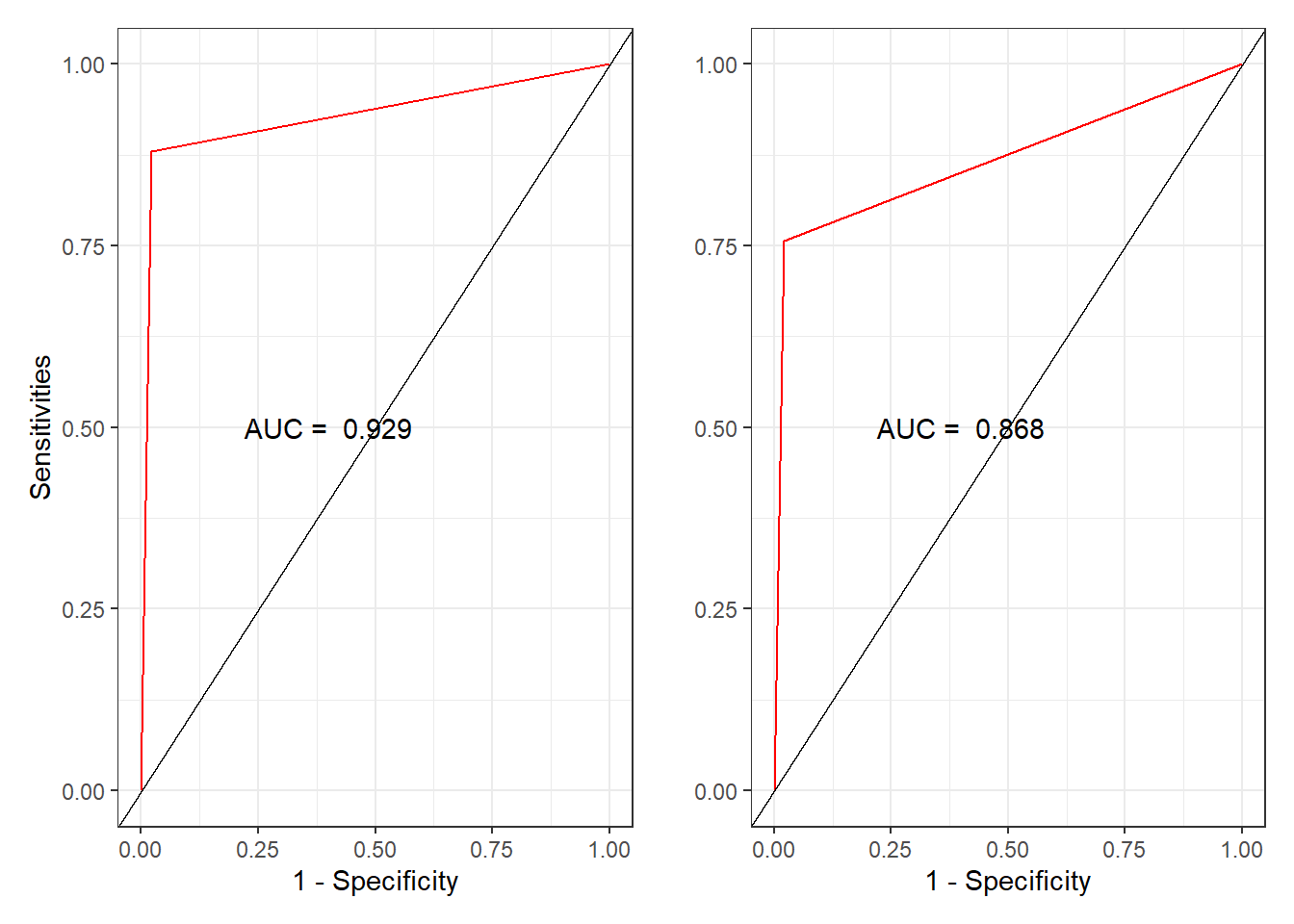
绘制ROC图形。
# 定义data = NULL声明未用任何数据 <- ggplot (data = NULL , aes (x = 1 - specificityRp, y = sensitivityRp)) + geom_line (color = "red" ) + geom_abline () + annotate ("text" , x = 0.4 , y = 0.5 , label = paste ("AUC = " , round (rocPart$ auc, 3 ))) + theme_bw () + labs (x = "1 - Specificity" , y = "Sensitivities" )<- ggplot (data = NULL , aes (x = 1 - specificityNb,y = sensitivityNb)) + geom_line (color = "red" ) + geom_abline () + annotate ("text" , x = 0.4 , y = 0.5 ,label = paste ("AUC = " ,round (rocNb$ auc, 3 ))) + theme_bw () + labs (x = "1 - Specificity" , y = " " )| pNb
(ref:fig-ROC)
从AUC值来看,同样是回归树模型的拟合效果好于朴素贝叶斯模型。
模型应用
使用回归树模型预测分类的概率,绘制交互预测表
# type = "prob"表示结果显示为概率
# predEnd <- predict(rpartmodel, testData[-7],
#                   type = "prob")

# 合并预测结果及概率
# dataEnd <- cbind(round(predEnd, 3), predRpart)

# 重命名预测结果表列名。
# names(dataEnd) <- c("pred.0", "pred.1", "pred")

# head(dataEnd)
# 生成交互式表格
# datatable(dataEnd)
mlr3建模
回归树模型
建立任务
<- read.csv ("data/HR_comma_sep.csv" )$ left <- factor (hr$ left)$ salary <- factor (hr$ salary)$ sales <- factor (hr$ sales)<- hr_model <- hr %>% filter (last_evaluation >= 0.70 | >= 4 | >= 5 )<- $ new (id = "left" , backend = hr_model,target = "left" )
<TaskClassif:left> (10394 x 10)
* Target: left
* Properties: twoclass
* Features (9):
  - int (5): Work_accident, average_montly_hours, number_project,
    promotion_last_5years, time_spend_company
  - dbl (2): last_evaluation, satisfaction_level
  - fct (2): salary, sales
定义学习器
<- lrn ("classif.rpart" , predict_type = "prob" )
基础训练+预测
set.seed (1234 )# 划分训练集和测试集 <- sample (task_hr$ nrow, 0.7 * task_hr$ nrow)<- setdiff (seq_len (task_hr$ nrow), train_set)# 训练模型 $ train (task_hr, row_ids = train_set)# 数据预测 <- learner_rpart$ predict (task_hr, row_ids = test_set)# 建立混淆矩阵 $ confusion
        truth
response    0    1
       0 2483   85
       1   17  534
# 评估模型准确性 <- msr ("classif.acc" ) $ score (measure_rpart)
重采样
# 自动重采样 ## 定义重采样方法:5折交叉 <- rsmp ("cv" , folds = 5L)## 应用重采样方法 <- resample (task_hr, learner_rpart, resampling_rpart)
INFO  [18:54:50.866] [mlr3] Applying learner 'classif.rpart' on task 'left' (iter 1/5)
INFO  [18:54:50.959] [mlr3] Applying learner 'classif.rpart' on task 'left' (iter 3/5)
INFO  [18:54:51.019] [mlr3] Applying learner 'classif.rpart' on task 'left' (iter 5/5)
INFO  [18:54:51.071] [mlr3] Applying learner 'classif.rpart' on task 'left' (iter 2/5)
INFO  [18:54:51.133] [mlr3] Applying learner 'classif.rpart' on task 'left' (iter 4/5)
## 每次重采样建模评分 $ score (measure_rpart)
                task task_id                   learner    learner_id
1: <TaskClassif[50]>    left <LearnerClassifRpart[38]> classif.rpart
2: <TaskClassif[50]>    left <LearnerClassifRpart[38]> classif.rpart
3: <TaskClassif[50]>    left <LearnerClassifRpart[38]> classif.rpart
4: <TaskClassif[50]>    left <LearnerClassifRpart[38]> classif.rpart
5: <TaskClassif[50]>    left <LearnerClassifRpart[38]> classif.rpart
           resampling resampling_id iteration              prediction
1: <ResamplingCV[20]>            cv         1 <PredictionClassif[20]>
2: <ResamplingCV[20]>            cv         2 <PredictionClassif[20]>
3: <ResamplingCV[20]>            cv         3 <PredictionClassif[20]>
4: <ResamplingCV[20]>            cv         4 <PredictionClassif[20]>
5: <ResamplingCV[20]>            cv         5 <PredictionClassif[20]>
   classif.acc
1:   0.9639250
2:   0.9735450
3:   0.9610390
4:   0.9672920
5:   0.9682387
## 将重采样的模型进行聚合并评分 $ aggregate (measure_rpart)
得到的回归树模型最终的拟合准确率为96.75%,拟合效果不错
朴素贝叶斯模型
建立任务
<- read.csv ("data/HR_comma_sep.csv" )$ left <- factor (hr$ left)$ salary <- factor (hr$ salary)$ sales <- factor (hr$ sales)<- hr_model <- hr %>% filter (last_evaluation >= 0.70 | >= 4 | >= 5 )<- $ new (id = "left" , backend = hr_model,target = "left" )
<TaskClassif:left> (10394 x 10)
* Target: left
* Properties: twoclass
* Features (9):
  - int (5): Work_accident, average_montly_hours, number_project,
    promotion_last_5years, time_spend_company
  - dbl (2): last_evaluation, satisfaction_level
  - fct (2): salary, sales
选择学习器
<- lrn ("classif.naive_bayes" ,predict_type = "prob" )
划分训练集和测试集
set.seed (1234 )<- sample (task_hr_nb$ nrow, task_hr_nb$ nrow * 0.7 )<- setdiff (seq_len (task_hr_nb$ nrow), train_set)
模型训练和预测
# 模型训练 $ train (task_hr_nb, row_ids = train_set)$ model # 查看训练好的模型
Naive Bayes Classifier for Discrete Predictors

Call:
naiveBayes.default(x = x, y = y)

A-priori probabilities:
y
        0         1
0.8074227 0.1925773

Conditional probabilities:
   Work_accident
y        [,1]      [,2]
  0 0.1813075 0.3853055
  1 0.0442541 0.2057326

   average_montly_hours
y       [,1]     [,2]
  0 201.0504 45.49460
  1 254.7744 34.45457

   last_evaluation
y        [,1]      [,2]
  0 0.7657457 0.1552908
  1 0.8763241 0.1013923

   number_project
y       [,1]     [,2]
  0 3.959993 1.023111
  1 5.244825 1.156665

   promotion_last_5years
y          [,1]       [,2]
  0 0.028770855 0.16717611
  1 0.002141328 0.04624142

   salary
y         high        low     medium
  0 0.10316650 0.44722506 0.44960844
  1 0.01641685 0.60314061 0.38044254

   sales
y   accounting         hr         IT management  marketing product_mng
  0 0.04902962 0.04324140 0.08614232 0.04971059 0.05498808  0.06179775
  1 0.05424697 0.04782298 0.07994290 0.02997859 0.04710921  0.05353319
   sales
y        RandD      sales    support  technical
  0 0.05720123 0.27221655 0.15253660 0.17313585
  1 0.03783012 0.26766595 0.15488936 0.22698073

   satisfaction_level
y        [,1]      [,2]
  0 0.6622302 0.2274002
  1 0.4660742 0.3465198

   time_spend_company
y       [,1]      [,2]
  0 3.654069 1.6892539
  1 4.559600 0.7978871
# 模型预测 <- learner_nb$ predict (task_hr_nb, row_ids = test_set)# 查看预测结果
<PredictionClassif> for 3119 observations:
    row_ids truth response       prob.0    prob.1
          2     1        1 0.0002953563 0.9997046
          3     1        1 0.1080414241 0.8919586
          4     1        1 0.0031520108 0.9968480
---
      10388     1        1 0.0423579034 0.9576421
      10390     1        0 0.5807408182 0.4192592
      10392     1        1 0.0014815943 0.9985184
模型评估
        truth
response    0    1
       0 2243  100
       1  257  519
<- msr ("classif.acc" )$ score (measure_nb) # 预测精度
重采样
<- rsmp ("cv" , folds = 5L)<- resample (task_hr_nb, learner_nb, resampling_nb)
INFO  [18:54:52.391] [mlr3] Applying learner 'classif.naive_bayes' on task 'left' (iter 1/5)
INFO  [18:54:52.820] [mlr3] Applying learner 'classif.naive_bayes' on task 'left' (iter 3/5)
INFO  [18:54:53.230] [mlr3] Applying learner 'classif.naive_bayes' on task 'left' (iter 5/5)
INFO  [18:54:53.634] [mlr3] Applying learner 'classif.naive_bayes' on task 'left' (iter 2/5)
INFO  [18:54:54.031] [mlr3] Applying learner 'classif.naive_bayes' on task 'left' (iter 4/5)
                task task_id                        learner          learner_id
1: <TaskClassif[50]>    left <LearnerClassifNaiveBayes[36]> classif.naive_bayes
2: <TaskClassif[50]>    left <LearnerClassifNaiveBayes[36]> classif.naive_bayes
3: <TaskClassif[50]>    left <LearnerClassifNaiveBayes[36]> classif.naive_bayes
4: <TaskClassif[50]>    left <LearnerClassifNaiveBayes[36]> classif.naive_bayes
5: <TaskClassif[50]>    left <LearnerClassifNaiveBayes[36]> classif.naive_bayes
           resampling resampling_id iteration              prediction
1: <ResamplingCV[20]>            cv         1 <PredictionClassif[20]>
2: <ResamplingCV[20]>            cv         2 <PredictionClassif[20]>
3: <ResamplingCV[20]>            cv         3 <PredictionClassif[20]>
4: <ResamplingCV[20]>            cv         4 <PredictionClassif[20]>
5: <ResamplingCV[20]>            cv         5 <PredictionClassif[20]>
   classif.acc
1:   0.8840789
2:   0.8951419
3:   0.8946609
4:   0.8869649
5:   0.8695861
$ aggregate (measure_nb)
通过两种模型的评估,我们发现回归树模型的拟合度比朴素贝叶斯更好,与传统方法得出的结论一致。
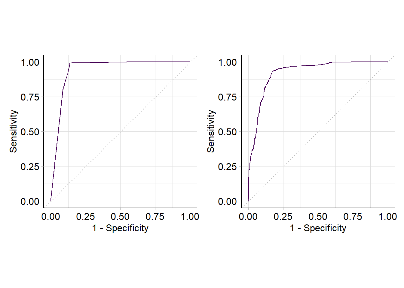
利用mlr3进行ROC曲线绘制
library (mlr3viz)<- autoplot (prediction_nb, type = "roc" )<- autoplot (prediction_rpart, type = "roc" )| roc_nb
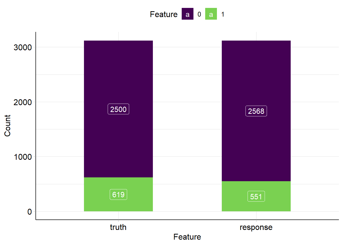
模型应用
使用回归树模型预测分类概率,绘制表格交互表
autoplot (prediction_rpart)
# type = "prob"表示结果显示为概率 <- predict (rpartmodel, testData[- 7 ],type = "prob" )# 合并预测结果及概率 <- cbind (round (predEnd, 3 ), predRpart)# 重命名预测结果表列名。 names (dataEnd) <- c ("pred.0" , "pred.1" , "pred" )# head(dataEnd) # 生成交互式表格 # datatable(dataEnd)